
OpenCV—Python 图像去模糊(维纳滤波,约束最小二乘方滤波)
文章目录一、维纳滤波二、约束最小二乘方滤波一、维纳滤波对于运动引起的图像模糊,最简单的方法是直接做逆滤波,但是逆滤波对加性噪声特别敏感,使得恢复的图像几乎不可用。最小均方差(维纳)滤波用来去除含有噪声的模糊图像,其目标是找到未污染图像的一个估计,使它们之间的均方差最小,可以去除噪声,同时清晰化模糊图像。y(t)=h(t)⨂x(t)+n(t)y(t)=h(t)\bigotimes x(t)+n...
一、维纳滤波
对于运动引起的图像模糊,最简单的方法是直接做逆滤波,但是逆滤波对加性噪声特别敏感,使得恢复的图像几乎不可用。最小均方差(维纳)滤波用来去除含有噪声的模糊图像,其目标是找到未污染图像的一个估计,使它们之间的均方差最小,可以去除噪声,同时清晰化模糊图像。
y
(
t
)
=
h
(
t
)
⨂
x
(
t
)
+
n
(
t
)
y(t)=h(t)\bigotimes x(t)+n(t)
y(t)=h(t)⨂x(t)+n(t)
-
其中:
-
⨂
\bigotimes
⨂ 是卷积符号
x ( t ) x(t) x(t) 是在时间 t t t 刻输入的信号(未知)
h ( t ) h(t) h(t) 是一个线性时间不变系统的脉冲响应(已知)
n ( t ) n(t) n(t) 是加性噪声,与 x ( t ) x(t) x(t)不相关(未知)
y ( t ) y(t) y(t) 是我们观察到的信号
我们的目标是找出这样的卷积函数 g ( t ) g(t) g(t),这样我们可以如下得到估计的 x ( t ) x(t) x(t)
x ^ ( t ) = g ( t ) ∗ y ( t ) \hat{x}(t)=g(t)∗y(t) x^(t)=g(t)∗y(t)
这里
x
^
(
t
)
\hat{x}(t)
x^(t)是
x
(
t
)
x(t)
x(t)的最小均方差估计。
基于这种误差度量, 滤波器可以在频率域如下描述
G
(
f
)
=
H
∗
(
f
)
S
(
f
)
∣
H
(
f
)
∣
2
S
(
f
)
+
N
(
f
)
=
H
∗
(
f
)
∣
H
(
f
)
∣
2
+
N
(
f
)
/
S
(
f
)
G(f)=\frac{H^∗(f)S(f)}{|H(f)|^2S(f)+N(f)}=\frac{H^∗(f)}{|H(f)|^2+N(f)/S(f)}
G(f)=∣H(f)∣2S(f)+N(f)H∗(f)S(f)=∣H(f)∣2+N(f)/S(f)H∗(f)
-
这里:
-
G
(
f
)
G(f)
G(f))和
H
(
f
)
H(f)
H(f)是
g
g
g和
h
h
h在频率域ff的傅里叶变换。
S ( f ) S(f) S(f)是输入信号 x ( t ) x(t) x(t) 的功率谱。
N ( f ) N(f) N(f)是噪声的 n ( t ) n(t) n(t) 的功率谱。
上标 ∗ ^∗ ∗ 代表复数共轭。
滤波过程可以在频率域完成: X ^ ( f ) = G ( f ) ∗ Y ( f ) \hat{X}(f)=G(f)∗Y(f) X^(f)=G(f)∗Y(f)
这里 X ^ ( f ) \hat{X}(f) X^(f) 是 x ^ ( t ) \hat{x}(t) x^(t)的傅里叶变换,通过逆傅里叶变化可以得到去卷积后的结果 x ^ ( t ) \hat{x}(t) x^(t)。
上面的式子可以改写成更为清晰的形式:
G
(
f
)
=
1
H
(
f
)
[
∣
H
(
f
)
∣
2
∣
H
(
f
)
∣
2
+
N
(
f
)
S
(
f
)
]
=
1
H
(
f
)
[
∣
H
(
f
)
∣
2
∣
H
(
f
)
∣
2
+
1
S
N
R
(
f
)
]
G(f) = \frac{1}{H(f)}\left [ \frac{|H(f)|^2}{|H(f)|^2 + \frac{N(f)}{S(f)}} \right ] = \frac{1}{H(f)}\left [ \frac{|H(f)|^2}{|H(f)|^2 + \frac{1}{SNR(f)}} \right ]
G(f)=H(f)1⎣⎡∣H(f)∣2+S(f)N(f)∣H(f)∣2⎦⎤=H(f)1[∣H(f)∣2+SNR(f)1∣H(f)∣2]
这里 H ( f ) H(f) H(f) 是 h h h 在频率域 f f f 的傅里叶变换。 S N R ( f ) = S ( f ) / N ( f ) SNR(f)=S(f)/N(f) SNR(f)=S(f)/N(f)是信号噪声比。当噪声为零时(即信噪比趋近于无穷),方括号内各项也就等于1,意味着此时刻维纳滤波也就简化成逆滤波过程。但是当噪声增加时,信噪比降低,方括号里面值也跟着降低。这说明,维纳滤波的带通频率依赖于信噪比。
代码示例:如下代码参考于【博主】,自己解决了对RGB图片的支持,与诸位共勉。
import matplotlib.pyplot as plt
import numpy as np
from numpy import fft
import math
import cv2
# 仿真运动模糊
def motion_process(image_size, motion_angle):
PSF = np.zeros(image_size)
print(image_size)
center_position = (image_size[0] - 1) / 2
print(center_position)
slope_tan = math.tan(motion_angle * math.pi / 180)
slope_cot = 1 / slope_tan
if slope_tan <= 1:
for i in range(15):
offset = round(i * slope_tan) # ((center_position-i)*slope_tan)
PSF[int(center_position + offset), int(center_position - offset)] = 1
return PSF / PSF.sum() # 对点扩散函数进行归一化亮度
else:
for i in range(15):
offset = round(i * slope_cot)
PSF[int(center_position - offset), int(center_position + offset)] = 1
return PSF / PSF.sum()
# 对图片进行运动模糊
def make_blurred(input, PSF, eps):
input_fft = fft.fft2(input) # 进行二维数组的傅里叶变换
PSF_fft = fft.fft2(PSF) + eps
blurred = fft.ifft2(input_fft * PSF_fft)
blurred = np.abs(fft.fftshift(blurred))
return blurred
def inverse(input, PSF, eps): # 逆滤波
input_fft = fft.fft2(input)
PSF_fft = fft.fft2(PSF) + eps # 噪声功率,这是已知的,考虑epsilon
result = fft.ifft2(input_fft / PSF_fft) # 计算F(u,v)的傅里叶反变换
result = np.abs(fft.fftshift(result))
return result
def wiener(input, PSF, eps, K=0.01): # 维纳滤波,K=0.01
input_fft = fft.fft2(input)
PSF_fft = fft.fft2(PSF) + eps
PSF_fft_1 = np.conj(PSF_fft) / (np.abs(PSF_fft) ** 2 + K)
result = fft.ifft2(input_fft * PSF_fft_1)
result = np.abs(fft.fftshift(result))
return result
def normal(array):
array = np.where(array < 0, 0, array)
array = np.where(array > 255, 255, array)
array = array.astype(np.int16)
return array
def main(gray):
channel = []
img_h, img_w = gray.shape[:2]
PSF = motion_process((img_h, img_w), 60) # 进行运动模糊处理
blurred = np.abs(make_blurred(gray, PSF, 1e-3))
result_blurred = inverse(blurred, PSF, 1e-3) # 逆滤波
result_wiener = wiener(blurred, PSF, 1e-3) # 维纳滤波
blurred_noisy = blurred + 0.1 * blurred.std() * \
np.random.standard_normal(blurred.shape) # 添加噪声,standard_normal产生随机的函数
inverse_mo2no = inverse(blurred_noisy, PSF, 0.1 + 1e-3) # 对添加噪声的图像进行逆滤波
wiener_mo2no = wiener(blurred_noisy, PSF, 0.1 + 1e-3) # 对添加噪声的图像进行维纳滤波
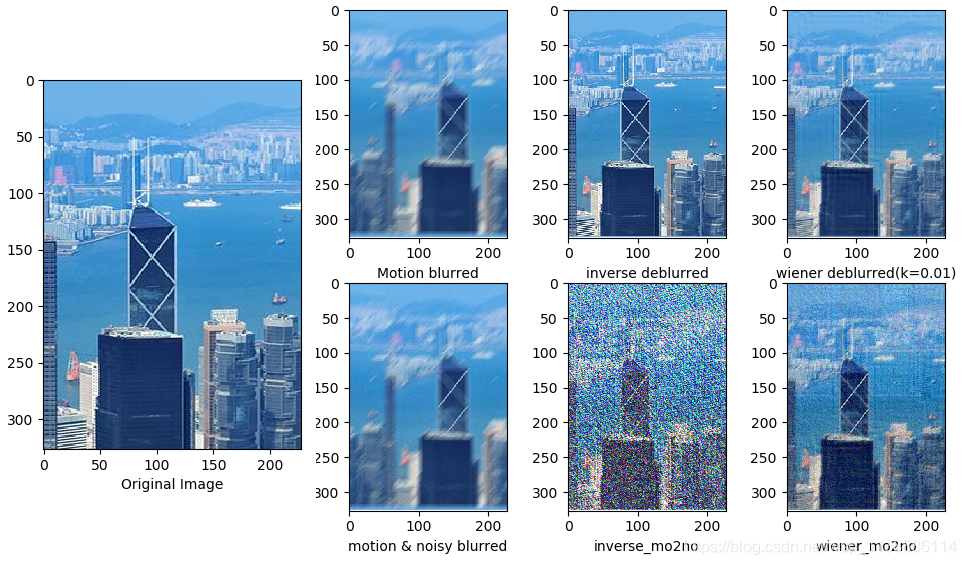
channel.append((normal(blurred),normal(result_blurred),normal(result_wiener),
normal(blurred_noisy),normal(inverse_mo2no),normal(wiener_mo2no)))
return channel
if __name__ == '__main__':
image = cv2.imread('./gggg/001.png')
b_gray, g_gray, r_gray = cv2.split(image.copy())
Result = []
for gray in [b_gray, g_gray, r_gray]:
channel = main(gray)
Result.append(channel)
blurred = cv2.merge([Result[0][0][0], Result[1][0][0], Result[2][0][0]])
result_blurred = cv2.merge([Result[0][0][1], Result[1][0][1], Result[2][0][1]])
result_wiener = cv2.merge([Result[0][0][2], Result[1][0][2], Result[2][0][2]])
blurred_noisy = cv2.merge([Result[0][0][3], Result[1][0][3], Result[2][0][3]])
inverse_mo2no = cv2.merge([Result[0][0][4], Result[1][0][4], Result[2][0][4]])
wiener_mo2no = cv2.merge([Result[0][0][5], Result[1][0][5], Result[2][0][5]])
#========= 可视化 ==========
plt.figure(1)
plt.xlabel("Original Image")
plt.imshow(np.flip(image, axis=2)) # 显示原图像
plt.figure(2)
plt.figure(figsize=(8, 6.5))
imgNames = {"Motion blurred":blurred,
"inverse deblurred":result_blurred,
"wiener deblurred(k=0.01)":result_wiener,
"motion & noisy blurred":blurred_noisy,
"inverse_mo2no":inverse_mo2no,
'wiener_mo2no':wiener_mo2no}
for i,(key,imgName) in enumerate(imgNames.items()):
plt.subplot(231+i)
plt.xlabel(key)
plt.imshow(np.flip(imgName, axis=2))
plt.show()
二、约束最小二乘方滤波
约束最小二乘方滤波(Constrained Least Squares Filtering,aka Tikhonov filtration,Tikhonov regularization)核心是H对噪声的敏感性问题。减少噪声敏感新问题的一种方法是以平滑度量的最佳复原为基础的,建立下列约束条件:
C
=
∑
0
M
−
1
∑
0
N
−
1
[
∇
2
f
(
x
,
y
)
]
2
C = \sum_0^{M-1}\sum_0^{N-1}[\nabla^2f(x,y)]^2
C=0∑M−10∑N−1[∇2f(x,y)]2
约束条件:
∣
∣
G
−
H
F
^
∣
∣
2
2
=
∣
∣
N
∣
∣
2
2
||G-H\hat{F}||_2^2 = ||N||_2^2
∣∣G−HF^∣∣22=∣∣N∣∣22
这里,
F
^
\hat{F}
F^是为退化图像的估计,
N
N
N为加性噪声,拉普拉斯算子
∇
2
\nabla^2
∇2在这里表示平滑程度。
推导:
将上式表示成矩阵形式,同时将约束项转换成拉格朗日乘子项:
∣
∣
P
F
^
∣
∣
2
2
−
λ
(
∣
∣
G
−
H
F
^
∣
∣
2
2
−
∣
∣
N
∣
∣
2
2
)
||P\hat{F}||_2^2 - \lambda \left ( ||G-H\hat{F}||_2^2 - ||N||_2^2 \right )
∣∣PF^∣∣22−λ(∣∣G−HF^∣∣22−∣∣N∣∣22)
最小化上代价函数,对
F
^
\hat{F}
F^求导,令等零有:
P
∗
P
F
^
=
λ
H
∗
(
G
−
H
F
^
)
P^∗P\hat{F}=λH^∗(G−H\hat{F})
P∗PF^=λH∗(G−HF^)
最后可得到:
F
^
=
λ
H
∗
G
λ
H
∗
H
+
P
∗
P
=
[
H
∗
∣
∣
H
∣
∣
2
2
+
λ
∣
∣
P
∣
∣
2
2
]
G
\hat{F} = \frac{ \lambda H^*G}{ \lambda H^*H + P^*P} = \left [ \frac{H^*}{||H||_2^2 + \lambda||P||_2^2 } \right ]G
F^=λH∗H+P∗PλH∗G=[∣∣H∣∣22+λ∣∣P∣∣22H∗]G
P
P
P是函数
P
=
[
0
−
1
0
−
1
4
−
1
0
−
1
0
]
P = \begin{bmatrix} 0 & -1 &0 \\ -1 & 4 &-1 \\ 0 & -1 & 0 \end{bmatrix}
P=⎣⎡0−10−14−10−10⎦⎤
三、psf2otf ,circShift
circshift(psf,K)
当K为一个数字时,只对矩阵进行上下平移,当K为一个坐标时,会对矩阵进行上下和左右两个方向进行平移。示例如下:
执行:平移坐标(-1,-1),对矩阵进行上移,左移1个单位,效果如下:
[
0
−
1
0
−
1
4
−
1
0
−
1
0
]
⇒
[
4
−
1
−
1
−
1
0
0
−
1
0
0
]
\begin{bmatrix} 0 & -1 & 0\\ -1 & 4 & -1\\ 0 & -1 & 0 \end{bmatrix} \Rightarrow \begin{bmatrix} 4 & -1 & -1\\ -1 & 0 & 0\\ -1 & 0 & 0 \end{bmatrix}
⎣⎡0−10−14−10−10⎦⎤⇒⎣⎡4−1−1−100−100⎦⎤
示例2:平移坐标(1,2),对矩阵进行下移1个单位,右移2个单位,效果如下:
[
1
2
3
4
5
6
7
8
9
10
11
12
13
14
15
16
17
18
19
20
]
⇒
[
19
20
16
17
18
4
5
1
2
3
9
10
6
7
8
14
15
11
12
13
]
\begin{bmatrix} 1& 2& 3& 4& 5\\ 6& 7& 8& 9& 10\\ 11&12&13&14&15\\ 16&17&18&19&20\\ \end{bmatrix} \Rightarrow \begin{bmatrix} 19&20&16&17&18\\ 4&5&1&2&3\\ 9&10&6&7&8\\ 14&15&11&12&13 \end{bmatrix}
⎣⎢⎢⎡1611162712173813184914195101520⎦⎥⎥⎤⇒⎣⎢⎢⎡1949142051015161611172712183813⎦⎥⎥⎤
psf2otf()
依次执行效果如下:
[
0
−
1
0
−
1
4
−
1
0
−
1
0
]
⇒
[
0.
+
0.
j
3.
+
0.
j
3.
+
0.
j
3.
+
0.
j
6.
+
0.
j
6.
+
0.
j
3.
+
0.
j
6.
+
0.
j
6.
+
0.
j
]
⇒
[
0
3
3
3
6
6
3
6
6
]
\begin{bmatrix} 0 & -1 & 0\\ -1 & 4 & -1\\ 0 & -1 & 0 \end{bmatrix} \Rightarrow \begin{bmatrix} 0.+0.j & 3.+0.j & 3.+0.j\\ 3.+0.j & 6.+0.j & 6.+0.j\\ 3.+0.j & 6.+0.j & 6.+0.j \end{bmatrix} \Rightarrow \begin{bmatrix} 0& 3& 3\\ 3 & 6 & 6\\ 3 & 6 & 6 \end{bmatrix}
⎣⎡0−10−14−10−10⎦⎤⇒⎣⎡0.+0.j3.+0.j3.+0.j3.+0.j6.+0.j6.+0.j3.+0.j6.+0.j6.+0.j⎦⎤⇒⎣⎡033366366⎦⎤
其中 np.fft.fft2()返回值为复数,可以用np.real()获取复数的实部,np.imag()用来获取虚部。
代码示例:自己用numpy重写了matlab里面的psf2otf这个函数,
下载地址:https://download.csdn.net/download/wsp_1138886114/11419292 。请原谅我这样做,我也想搞点积分用。
或者查看:https://blog.csdn.net/wsp_1138886114/article/details/97611270
# coding: utf-8
import numpy as np
import matplotlib.pyplot as plt
from numpy import fft
import cv2
from temp_004 import psf2otf
def motion_blur(gray, degree=7, angle=60):
gray = np.array(gray)
M = cv2.getRotationMatrix2D((round(degree / 2), round(degree / 2)), angle, 1)
motion_blur_kernel = np.diag(np.ones(degree))
motion_blur_kernel = cv2.warpAffine(motion_blur_kernel, M, (degree, degree))
PSF = motion_blur_kernel / degree
blurred = cv2.filter2D(gray, -1, PSF)
blurred = cv2.normalize(blurred,None, 0, 255, cv2.NORM_MINMAX)
blurred = np.array(blurred, dtype=np.uint8)
return blurred,PSF
def inverse(blurred, PF):
IF_fft = fft.fft2(blurred)
result = fft.ifft2(IF_fft / PF)
result = np.real(result)
return result
def wiener(blurred, PF, SNR=0.01): # 维纳滤波,K=0.01
IF_fft = fft.fft2(blurred)
G_f = np.conj(PF) / (np.abs(PF) ** 2 + SNR)
result = fft.ifft2(IF_fft * G_f)
result = np.real(result)
return result
def CLSF(blurred,PF,gamma = 0.05):
outheight, outwidth = blurred.shape[:2]
kernel = np.array([[0, -1, 0],
[-1, 4, -1],
[0, -1, 0]])
PF_kernel = psf2otf(kernel,[outheight, outwidth])
IF_noisy = fft.fft2(blurred)
numerator = np.conj(PF)
denominator = PF**2 + gamma*(PF_kernel**2)
CLSF_deblurred = fft.ifft2(numerator* IF_noisy/ denominator)
CLSF_deblurred = np.real(CLSF_deblurred)
return CLSF_deblurred
def normal(array):
array = np.where(array < 0, 0, array)
array = np.where(array > 255, 255, array)
array = array.astype(np.int16)
return array
def main(gray):
channel = []
img_H, img_W = gray.shape[:2]
blurred,PSF = motion_blur(gray, degree=15, angle=30) # 进行运动模糊处理
PF = psf2otf(PSF, [img_H, img_W])
inverse_blurred =normal(inverse(blurred, PF)) # 逆滤波
wiener_blurred = normal(wiener(blurred, PF)) # 维纳滤波
CLSF_blurred = normal(CLSF(blurred, PF)) # 约束最小二乘方滤波
blurred_noisy = blurred + 0.1 * blurred.std() * \
np.random.standard_normal(blurred.shape) # 添加噪声
inverse_noise = normal(inverse(blurred_noisy, PF)) # 添加噪声-逆滤波
wiener_noise = normal(wiener(blurred_noisy, PF)) # 添加噪声-维纳滤波
CLSF_noise = normal(CLSF(blurred_noisy, PF)) # 添加噪声-约束最小二乘方滤波
print('CLSF_deblurred',CLSF_blurred)
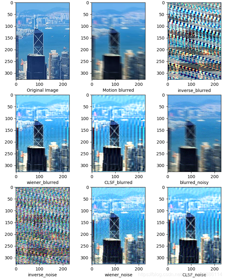
channel.append((blurred,inverse_blurred,wiener_blurred,CLSF_blurred,
normal(blurred_noisy),inverse_noise,wiener_noise,CLSF_noise))
return channel
if __name__ == '__main__':
image = cv2.imread('./gggg/001.png')
b_gray, g_gray, r_gray = cv2.split(image.copy())
Result = []
for gray in [b_gray, g_gray, r_gray]:
channel = main(gray)
Result.append(channel)
blurred = cv2.merge([Result[0][0][0], Result[1][0][0], Result[2][0][0]])
inverse_blurred = cv2.merge([Result[0][0][1], Result[1][0][1], Result[2][0][1]])
wiener_blurred = cv2.merge([Result[0][0][2], Result[1][0][2], Result[2][0][2]])
CLSF_blurred = cv2.merge([Result[0][0][3], Result[1][0][3], Result[2][0][3]])
blurred_noisy = cv2.merge([Result[0][0][4], Result[1][0][4], Result[2][0][4]])
inverse_noise = cv2.merge([Result[0][0][5], Result[1][0][5], Result[2][0][5]])
wiener_noise = cv2.merge([Result[0][0][6], Result[1][0][6], Result[2][0][6]])
CLSF_noise = cv2.merge([Result[0][0][7], Result[1][0][7], Result[2][0][7]])
#========= 可视化 ==========
plt.figure(figsize=(9, 11))
plt.gray()
imgNames = {"Original Image":image,
"Motion blurred":blurred,
"inverse_blurred":inverse_blurred,
"wiener_blurred": wiener_blurred,
"CLSF_blurred": CLSF_blurred,
'blurred_noisy': blurred_noisy,
"inverse_noise":inverse_noise,
"wiener_noise":wiener_noise,
"CLSF_noise":CLSF_noise
}
for i,(key,imgName) in enumerate(imgNames.items()):
plt.subplot(331+i)
plt.xlabel(key)
plt.imshow(np.flip(imgName, axis=2))
plt.show()
鸣谢
傅里叶变换:https://blog.csdn.net/a13602955218/article/details/84448075
https://blog.csdn.net/bluecol/article/details/47357717
https://blog.csdn.net/bluecol/article/details/46242355
https://blog.csdn.net/qq_29769263/article/details/85330933
特别鸣谢
https://blog.csdn.net/baimafujinji/article/details/73882265
https://blog.csdn.net/bluecol/article/details/47359421
https://blog.csdn.net/bingbingxie1/article/details/79398601

旨在为数千万中国开发者提供一个无缝且高效的云端环境,以支持学习、使用和贡献开源项目。
更多推荐


 60
60 0
0- 0


 已为社区贡献14条内容

所有评论(0)