
阵列信号处理笔记(2):均匀线阵、均匀加权线阵、波束方向图
阵列信号处理笔记第2篇。
阵列信号处理笔记(2)
文章目录
均匀线阵(Uniform Linear Array)

均匀线阵是一个具有均匀阵元间隔的线性阵列,为了方便推导,设阵元全部位于Z轴上,且阵列中心位于坐标原点,因此阵元的坐标都可以简洁的表示为
p
n
=
(
0
,
0
,
p
z
n
)
T
\mathbf{p}_n=\left( 0,0,p_{z_n} \right)^T
pn=(0,0,pzn)T,其中
p
z
n
=
(
n
−
N
−
1
2
)
d
,
n
∈
{
0
,
1
,
.
.
.
,
N
−
1
}
(1)
p_{z_n}=\left( n-\frac{N-1}{2} \right)d,\quad n\in \left\{ 0,1,...,N-1 \right\}\tag{1}
pzn=(n−2N−1)d,n∈{0,1,...,N−1}(1)
通常来说这个阵元间距
d
d
d取
λ
/
2
\lambda/2
λ/2[注1],也就是半波长。
[注1]
这个参数不是瞎特喵取的,还是有一定道理滴…这个主要涉及到空域的采样。为了简化模型,假设阵元水平排布且间隔为 d d d,考虑理想线阵的一个窄带远场响应(主要为了近似为一个平面波,并用延迟-求和模型描述),波面法向量与水平面夹角为 θ \theta θ。
可以看到,平面波依次到达阵元,相当于依次对平面波做采样,其采样间隔(距离)非常容易计算,为 d cos θ d \cos \theta dcosθ,类比幼儿园学习到的奈奎斯特采样定理,采样率至少要大于信号的2倍最高频,也就是采样周期要低于信号最小周期的一半,那么自然有
∣ d cos θ ∣ ⩽ λ 2 ∀ θ ∈ [ 0 , π ] \left| d \cos \theta \right| \leqslant \frac{\lambda}{2}\quad \forall \theta \in \left[ 0, \pi \right] ∣dcosθ∣⩽2λ∀θ∈[0,π]这个极限情况是当 θ = 0 \displaystyle \theta=0 θ=0或 θ = π \displaystyle \theta=\pi θ=π时,为了保证上面那个不等式恒成立,最经济的做法就是取 d = λ 2 \displaystyle d=\frac{\lambda}{2} d=2λ。其实不难发现,当 θ \theta θ越接近 π 2 \displaystyle\frac{\pi}{2} 2π,空域采样的频率就越高,越靠近 θ = 0 \displaystyle \theta=0 θ=0或 θ = π \displaystyle \theta=\pi θ=π时采样率越接近奈奎斯特频率…所以从某种意义上来说,做一些beamforming或者是DoA estimation的时候,这种非常临界的角度出来的效果往往不太好。

由上一篇博文的内容可知,阵列流形矢量可以表示为
v
(
k
)
=
(
e
−
j
k
T
p
0
e
−
j
k
T
p
1
⋮
e
−
j
k
T
p
N
−
1
)
(2)
\mathbf{v}(\mathbf{k})=\left(\begin{array}{c} e^{-j\mathbf{k}^T \mathbf{p}_0}\\e^{-j\mathbf{k}^T \mathbf{p}_1}\\\vdots\\e^{-j\mathbf{k}^T \mathbf{p}_{N-1}} \end{array}\right)\tag{2}
v(k)=
e−jkTp0e−jkTp1⋮e−jkTpN−1
(2)
这里
k
=
(
k
x
k
y
k
z
)
=
−
2
π
λ
(
sin
θ
cos
ϕ
sin
θ
sin
ϕ
cos
θ
)
(3)
\mathbf{k}=\left(\begin{array}{c} k_x\\k_y\\k_z \end{array}\right)=-\frac{2 \pi}{\lambda}\left(\begin{array}{c} \sin \theta \cos \phi \\\sin \theta \sin \phi \\\cos \theta \end{array}\right)\tag{3}
k=
kxkykz
=−λ2π
sinθcosϕsinθsinϕcosθ
(3)
带入阵列流形矢量不难得到
v
(
k
)
=
(
e
j
(
N
−
1
2
)
k
z
d
e
j
(
N
−
1
2
−
1
)
k
z
d
⋮
e
−
j
(
N
−
1
2
)
k
z
d
)
(4)
\mathbf{v}(\mathbf{k})=\left(\begin{array}{c} e^{j\left( \frac{N-1}{2} \right)k_zd}\\e^{j\left( \frac{N-1}{2} -1\right)k_zd}\\\vdots\\e^{-j\left( \frac{N-1}{2} \right)k_zd} \end{array}\right)\tag{4}
v(k)=
ej(2N−1)kzdej(2N−1−1)kzd⋮e−j(2N−1)kzd
(4)
其实这意味着ULA仅有一个方向的分辨能力。于是整个阵列的频率-波数响应
γ
(
w
,
k
)
\mathbf{\gamma}(w,\mathbf{k})
γ(w,k)可以表示为
γ
(
w
,
k
)
=
ω
H
v
(
k
)
=
∑
n
=
0
N
−
1
w
n
∗
e
−
j
(
n
−
N
−
1
2
)
k
z
d
(5)
\mathbf{\gamma}(w,\mathbf{k})= \mathbf{\omega}^\mathrm{H}\mathbf{v}(k)=\sum _{n=0} ^{N-1}w_n^*e^{-j\left( n-\frac{N-1}{2} \right)k_zd}\tag{5}
γ(w,k)=ωHv(k)=n=0∑N−1wn∗e−j(n−2N−1)kzd(5)
其中
w
n
w_n
wn是各个阵列的频域加权系数,用共轭转置主要是为了后面章节的推导比较自然。这里介绍另外两种阵列流形和频率-波数响应的表示法。一种是利用式3中,波数分量与方向向量之间的关系,可以得到
θ
\theta
θ空间的响应,也就是
γ
(
θ
)
=
ω
H
v
(
θ
)
=
∑
n
=
0
N
−
1
w
n
∗
e
−
j
(
n
−
N
−
1
2
)
2
π
λ
cos
θ
d
,
(6)
\mathbf{\gamma}(\theta)=\mathbf{\omega}^\mathrm{H}\mathbf{v}(\theta)=\sum _{n=0} ^{N-1}w_n^*e^{-j\left( n-\frac{N-1}{2} \right)\frac{2 \pi}{\lambda}\cos \theta d},\quad \tag{6}
γ(θ)=ωHv(θ)=n=0∑N−1wn∗e−j(n−2N−1)λ2πcosθd,(6)
或令
−
k
z
d
=
ψ
\displaystyle -k_zd=\psi
−kzd=ψ,得到
ψ
\psi
ψ域的频率-波数响应
γ
(
ψ
)
=
ω
H
v
(
ψ
)
=
∑
n
=
0
N
−
1
w
n
∗
e
j
(
n
−
N
−
1
2
)
ψ
,
(7)
\mathbf{\gamma}(\psi)=\mathbf{\omega}^\mathrm{H}\mathbf{v}(\psi)=\sum _{n=0} ^{N-1}w_n^*e^{j\left( n-\frac{N-1}{2} \right)\psi},\quad \tag{7}
γ(ψ)=ωHv(ψ)=n=0∑N−1wn∗ej(n−2N−1)ψ,(7)
这三种表示方法各有特点,其中波数域的表示更加接近第一性原理,物理意义明确。
θ
\theta
θ域的表示能直观反应阵列的方向特性,而
ψ
\psi
ψ域的比较离谱,他的形式比较接近某种意义上的Z变换(或者说DTFT),比如
γ
(
ψ
)
=
e
j
(
−
N
−
1
2
)
ψ
(
∑
n
=
0
N
−
1
w
n
e
j
n
ψ
)
∗
=
z
−
N
−
1
2
W
∗
(
z
)
∣
z
=
e
j
ψ
,
(8)
\mathbf{\gamma}(\psi)=e^{j\left( -\frac{N-1}{2} \right)\psi}\left( \sum _{n=0} ^{N-1}w_ne^{jn\psi} \right)^*=z^{-\frac{N-1}{2}}W^*(z)|_{z=e^{j \psi}},\quad \tag{8}
γ(ψ)=ej(−2N−1)ψ(n=0∑N−1wnejnψ)∗=z−2N−1W∗(z)∣z=ejψ,(8)
这种表示方法在分析上比较方便,后面很多推导都是直接在(8)上进行的。而利用DTFT的奇偶虚实性不然得到
ψ
\psi
ψ域频率-波数响应的一些性质,很多关于数字信号处理的知识能用进来,这里不再赘述。
另外还有一个u域的响应,这里令
u
=
cos
θ
u=\cos \theta
u=cosθ,并带入(8)得
γ
(
u
)
=
∑
n
=
0
N
−
1
w
n
∗
e
−
j
(
n
−
N
−
1
2
)
2
π
λ
u
d
,
(9)
\mathbf{\gamma}(u)=\sum _{n=0} ^{N-1}w_n^*e^{-j\left( n-\frac{N-1}{2} \right)\frac{2 \pi}{\lambda}u d},\quad \tag{9}
γ(u)=n=0∑N−1wn∗e−j(n−2N−1)λ2πud,(9)
根据奥卡姆剃刀原理,如非必要勿增实体,现在喵的搞了这么多乱七八糟的东西挺头大的…不过这些在后面推导中还是有用处的。
均匀加权线阵
均匀加权线阵是ULA的一个特例,其 w n = 1 N \displaystyle w_n=\frac{1}{N} wn=N1,对于这种ULA仔细分析是有必要的。考虑 ψ \psi ψ域的响应 γ ( ψ ) \mathbf{\gamma}(\psi) γ(ψ),显然无论N的奇偶,这是这个响应必然是一个实偶函数。
[注2] 简短的证明。
γ ( ψ ) = ω H v ( ψ ) = ω T v ( ψ ) = γ ∗ ( − ψ ) \mathbf{\gamma}(\psi)=\mathbf{\omega}^\mathrm{H}\mathbf{v}(\psi)= \mathbf{\omega}^\mathrm{T}\mathbf{v}(\psi)=\mathbf{\gamma}^*(-\psi) γ(ψ)=ωHv(ψ)=ωTv(ψ)=γ∗(−ψ)
而
γ ( ψ ) = J ω H v ( ψ ) = γ ( − ψ ) \mathbf{\gamma}(\psi)=\mathbf{J}\mathbf{\omega}^\mathrm{H}\mathbf{v}(\psi)= \mathbf{\gamma}(-\psi) γ(ψ)=JωHv(ψ)=γ(−ψ)
其中 J \mathbf{J} J为相应阶数的副对角阵,综上这是一个实偶函数。
将
w
n
=
1
N
\displaystyle w_n=\frac{1}{N}
wn=N1带入(7)中可得
γ
(
ψ
)
=
1
N
sin
(
N
ψ
/
2
)
sin
(
ψ
/
2
)
(9)
\mathbf{\gamma}(\psi)=\frac{1}{N}\frac{\sin \left( N \psi/2 \right)}{\sin \left( \psi/2 \right)}\tag{9}
γ(ψ)=N1sin(ψ/2)sin(Nψ/2)(9)
同理可以得到k域和
θ
\theta
θ域的响应。使用MATLAB对
ψ
\psi
ψ域的响应进行仿真,取波长为单位长,阵元数量为5,10,15,20,得到的结果如图所示。

clc;
clear;
close all;

[psi, B_5] = Calc_B(5);
[~, B_10] = Calc_B(10);
[~, B_15] = Calc_B(15);
[~, B_20] = Calc_B(20);

figure('Color','white','Name','frequency-wavenumber response','NumberTitle','off','Position', [500,500,800,480]);
plot(subplot(2,2,1), psi, B_5,'b-');Graph_Set(gca,[-8 8],[-0.28 1],'\psi','','N=5');
plot(subplot(2,2,2), psi, B_10,'b-');Graph_Set(gca,[-8 8],[-1 1],'\psi','','N=10');
plot(subplot(2,2,3), psi, B_15,'b-');Graph_Set(gca,[-8 8],[-0.28 1],'\psi','','N=15');
plot(subplot(2,2,4), psi, B_20,'b-');Graph_Set(gca,[-8 8],[-1 1],'\psi','','N=20');

function [psi, B] = Calc_B(N)
    n = (0 : N - 1);
    lambda = 1;
    d = lambda / 2;
    psi = (-8 : 0.001 : 8);
    V_psi = exp(-1i * (n - (N - 1) / 2)' * psi);
    B = real(ones(1, N) * V_psi / N);
end
function Graph_Set(ax,XLim,YLim,Xlabel,Ylabel,Title)
	ax.FontSize = 11;
	ax.Title.String = Title;
	ax.XLabel.String = Xlabel;
	ax.YLabel.String = Ylabel;
	ax.XLim = XLim;
	ax.YLim = YLim;
	ax.XGrid = 'on';
	ax.YGrid = 'on';
	ax.XMinorTick = 'on';
	ax.YMinorTick = 'on';
end
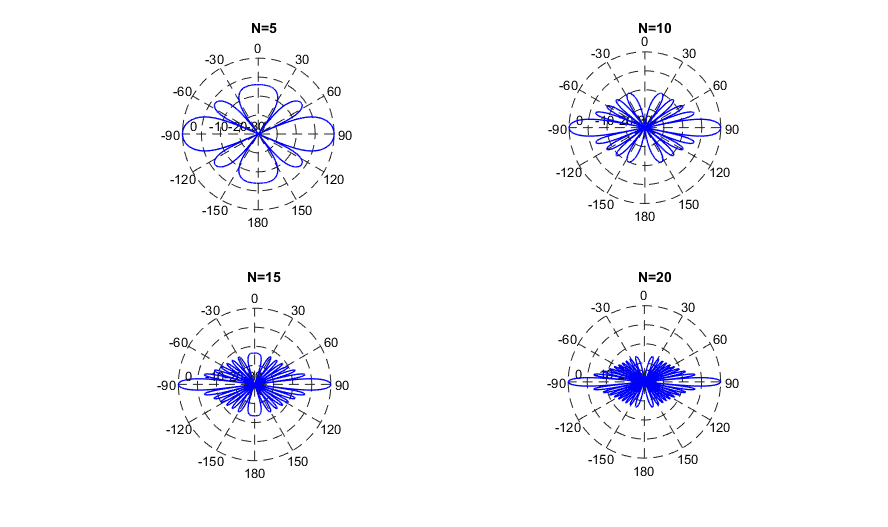
使用MATLAB对 θ \theta θ域的响应进行仿真,取波长为单位长,阵元数量为5,10,15,20,得到的结果如图所示,图看起来有点小啊。。。

clc;
clear;
close all;

[theta, G_5] = Calc_G(5);
[~, G_10] = Calc_G(10);
[~, G_15] = Calc_G(15);
[~, G_20] = Calc_G(20);

figure('Color','white','Name','frequency-wavenumber response','NumberTitle','off','Position', [500,500,800,480])
subplot(2,2,1); polardb(theta,G_5,-40,'b-'); title('N=5')
subplot(2,2,2); polardb(theta,G_10,-40,'b-');title('N=10')
subplot(2,2,3); polardb(theta,G_15,-40,'b-');title('N=15')
subplot(2,2,4); polardb(theta,G_20,-40,'b-');title('N=20')


function [theta, G_dB] = Calc_G(N)
    n = (0 : N - 1);
    lambda = 1;
    d = lambda / 2;
    theta = (0 : 0.001 : 2 * pi);
    V_theta = exp(-1i * (n - (N - 1) / 2)' * 2 * pi / lambda * cos(theta) * d);
    G_dB = 20 * log10(abs(ones(1, N) * V_theta / N));
end
这里用到了一个函数叫做polardb是MATLAB没有的。这个函数是99年K. Bell改编自MATLAB的Polar函数,代码贴在后面了。
波束方向图的关键参数
我们熟知,对于均匀加权ULA,其
ψ
\psi
ψ域的响应为
γ
(
ψ
)
=
1
N
sin
(
N
ψ
/
2
)
sin
(
ψ
/
2
)
\mathbf{\gamma}(\psi)=\frac{1}{N}\frac{\sin \left( N \psi/2 \right)}{\sin \left( \psi/2 \right)}
γ(ψ)=N1sin(ψ/2)sin(Nψ/2)

与滤波器之类的设计一样,我们也关心其响应的半功率波束带宽(HPBW,或者说3dB带宽)与第一过零点带宽(
B
W
N
N
BW_{NN}
BWNN)。半功率波束带宽是指其幅度下降到
2
2
\displaystyle\frac{\sqrt{2}}{2}
22时候的信号带宽,或者功率(幅度平方)下降到
1
2
\displaystyle\frac{1}{2}
21的带宽,其实也就是解这个方程
(
1
N
sin
(
N
ψ
/
2
)
sin
(
ψ
/
2
)
)
2
=
1
2
\left(\frac{1}{N}\frac{\sin \left( N \psi/2 \right)}{\sin \left( \psi/2 \right)} \right)^2=\frac{1}{2}
(N1sin(ψ/2)sin(Nψ/2))2=21
这东西是个超越方程,真TMD不好算。。。但是我们可以用一些手段得到数值解,例如经典的牛顿迭代法
牛顿迭代公式为: x n + 1 = x n − f ( x n ) / f ′ ( x n ) x_{n+1} = x_n - f(x_n) / f'(x_n) xn+1=xn−f(xn)/f′(xn),其中 f ′ ( x n ) f'(x_n) f′(xn) 表示 f ( x ) f(x) f(x) 在 x n x_n xn 处的导数。具体步骤如下:
- 初始化初始值 x 0 x_0 x0;
- 计算 f ( x 0 ) f(x_0) f(x0)和 f ′ ( x 0 ) f'(x_0) f′(x0);
- 使用牛顿迭代公式计算下一个近似解 x 1 = x 0 − f ( x 0 ) / f ′ ( x 0 ) x_1 = x_0 - f(x_0) / f'(x_0) x1=x0−f(x0)/f′(x0);
- 判断迭代停止条件,例如设定一个允许的误差范围 ε \varepsilon ε,当 ∣ x 1 − x 0 ∣ < ε |x_1 - x_0|<\varepsilon ∣x1−x0∣<ε 时停止迭代;
- 如果不满足停止条件,将 x 1 x_1 x1 赋值给 x 0 x_0 x0,回到步骤 2,继续进行迭代计算;
- 当满足停止条件时,近似解为 x 1 x_1 x1。
需要注意的是,牛顿迭代法可能会收敛到局部解,所以选择合适的初始值非常重要。
但实际上结束Mathematica强大的符号运算功能,解这种方程真是小case…但是需要注意的是,直接使用这段代码
NSolve[(1/N*Sin[N/2*p]/Sin[p/2])^2 == 0.5, p]
会给出实数域和复数域的解。这里有个小技巧,其实不难发现,随着
N
→
0
N\to 0
N→0,HPBW是趋于0的,故我们可以把
∣
γ
(
ψ
)
∣
2
|\gamma(\psi)|^2
∣γ(ψ)∣2在0点做泰勒展开,然后使用NSolve求解这个多项式方程,这样可以避免一些超越方程漏解的问题(对于这个方程MMA都能给到正确的解)。所以在这里直接不讲武德展到第10项,截断高次项得到一个多项式函数
f
(
ψ
)
=
1
12
(
1
−
N
2
)
ψ
2
+
(
N
6
360
−
N
4
144
+
N
2
240
)
ψ
4
N
2
+
(
−
N
8
20160
+
N
6
4320
−
N
4
2880
+
N
2
6048
)
ψ
6
N
2
+
(
N
10
1814400
−
N
8
241920
+
N
6
86400
−
N
4
72576
+
N
2
172800
)
ψ
8
N
2
+
(
−
N
12
239500800
+
N
10
21772800
−
N
8
4838400
+
N
6
2177280
−
N
4
2073600
+
N
2
5322240
)
ψ
10
N
2
+
1
f(\psi)=\frac{1}{12} \left(1-N^2\right) \psi^2+\frac{\left(\frac{N^6}{360}-\frac{N^4}{144}+\frac{N^2}{240}\right) \psi^4}{N^2}+\frac{\left(-\frac{N^8}{20160}+\frac{N^6}{4320}-\frac{N^4}{2880}+\frac{N^2}{6048}\right) \psi^6}{N^2}+\frac{\left(\frac{N^{10}}{1814400}-\frac{N^8}{241920}+\frac{N^6}{86400}-\frac{N^4}{72576}+\frac{N^2}{172800}\right) \psi^8}{N^2}+\frac{\left(-\frac{N^{12}}{239500800}+\frac{N^{10}}{21772800}-\frac{N^8}{4838400}+\frac{N^6}{2177280}-\frac{N^4}{2073600}+\frac{N^2}{5322240}\right) \psi^{10}}{N^2}+1
f(ψ)=121(1−N2)ψ2+N2(360N6−144N4+240N2)ψ4+N2(−20160N8+4320N6−2880N4+6048N2)ψ6+N2(1814400N10−241920N8+86400N6−72576N4+172800N2)ψ8+N2(−239500800N12+21772800N10−4838400N8+2177280N6−2073600N4+5322240N2)ψ10+1
注意这个函数是关于阵元数量N的,令
f
(
ψ
)
=
0
f(\psi)=0
f(ψ)=0,取大于0的第一个实根
ψ
^
\hat{\psi}
ψ^,那么很显然根据对称性HPBW=
2
ψ
^
2 \hat{\psi}
2ψ^。可以确定的是
ψ
^
\hat{\psi}
ψ^是一个与N有关的函数,可以看一下
ψ
^
\hat{\psi}
ψ^和N之间的关系。

这大致像一个反比例函数,所以可以尝试用MATLAB做一个函数拟合(拟合数据见文后),拟合表达式是 ψ ^ = a / N + b \hat{\psi}=a/N+b ψ^=a/N+b,当 N < 30 N<30 N<30的时候, ψ ^ = 2.8038 / N + 0.00092 \hat{\psi}=2.8038/N+0.00092 ψ^=2.8038/N+0.00092是一个比较精确的结果,当N>30时, ψ ^ = 2.7839 / N + 4.893 × 1 0 − 6 \hat{\psi}=2.7839/N+4.893\times 10^{-6} ψ^=2.7839/N+4.893×10−6是比较准确滴,不管怎么样,这里的b都是非常小的数,可以忽略。为了与 θ \theta θ域、 k k k域, u u u域表示联系起来,这里从系数a中提一个 π \pi π出来,得到下表。
| 空间 | N<30 | N>30 |
|---|---|---|
| ψ \psi ψ | 0.891 2 π N \displaystyle 0.891 \frac{2\pi}{N} 0.891N2π | 0.866 2 π N \displaystyle 0.866 \frac{2\pi}{N} 0.866N2π |
| θ \theta θ | 0.891 λ N d \displaystyle 0.891 \frac{\lambda}{Nd} 0.891Ndλ | 0.866 λ N d \displaystyle 0.866 \frac{\lambda}{Nd} 0.866Ndλ |
| u u u | 0.891 λ N d \displaystyle 0.891 \frac{\lambda}{Nd} 0.891Ndλ | 0.866 λ N d \displaystyle 0.866 \frac{\lambda}{Nd} 0.866Ndλ |
| k k k | 0.891 2 π N d \displaystyle 0.891 \frac{2\pi}{Nd} 0.891Nd2π | 0.866 2 π N d \displaystyle 0.866 \frac{2\pi}{Nd} 0.866Nd2π |
而 B W N N BW_{NN} BWNN的计算则要简单得多,主要就是看分子的零点情况。
| 空间 | B W N N BW_{NN} BWNN |
|---|---|
| ψ \psi ψ | 4 π N \displaystyle \frac{4\pi}{N} N4π |
| θ \theta θ | 2 λ N d \displaystyle\frac{2\lambda}{Nd} Nd2λ |
| u u u | 2 λ N d \displaystyle \frac{2\lambda}{Nd} Nd2λ |
| k k k | 4 π N d \displaystyle \frac{4\pi}{Nd} Nd4π |
附
polardb.m
%%%%%%%%%%%%%%%%%%%%%%%%%%%%%%%%
% polardb.m
% modified from Matlab's polar.m by K. Bell
% Last updated 8/30/00 by K. Bell
%%%%%%%%%%%%%%%%%%%%%%%%%%%%%%%%

function hpol=polardb(theta,rho,lim,line_style)
% polardb(theta,rho,lim,linestyle)
% Polardb is a modified version of the regular 'polar' function.
% Plotting range is -180 to 180 deg with zero at top.
% Theta increases in clockwise manner.
% Inputs:
%   theta - angles in RADIANS (although axes labeled in degrees)
%   rho   - plot value in dB
%   lim   - lower limit for plot in dB (e.g. -40)
%   line_style - string indicating line style, e.g. '-g' (optional)
% Example polardb(theta,beampatt,-40,'-r')
%
%POLAR	Polar coordinate plot.
%	POLAR(THETA, RHO) makes a plot using polar coordinates of
%	the angle THETA, in radians, versus the radius RHO.
%	POLAR(THETA,RHO,S) uses the linestyle specified in string S.
%	See PLOT for a description of legal linestyles.
%
%	See also PLOT, LOGLOG, SEMILOGX, SEMILOGY.

%	Copyright (c) 1984-94 by The MathWorks, Inc.

const=0.7;

if nargin < 3
	error('Requires 3 or 4 input arguments.')
elseif nargin == 3
        [n,n1]=size(theta);
	if isstr(rho)
		line_style = rho;
		rho = theta;
		[mr,nr] = size(rho);
		if mr == 1
			theta = 1:nr;
		else
			th = (1:mr)';
			theta = th(:,ones(1,nr));
		end
	else
		line_style = 'auto';
	end
elseif nargin == 2
	line_style = 'auto';
	rho = theta;
	[mr,nr] = size(rho);
	if mr == 1
		theta = 1:nr;
	else
		th = (1:mr)';
		theta = th(:,ones(1,nr));
	end
end
if isstr(theta) | isstr(rho)
	error('Input arguments must be numeric.');
end
if any(size(theta) ~= size(rho))
	error('THETA and RHO must be the same size.');
end

nr = size(rho,2);
tck = -floor(lim/10);
lim = -tck*10;
I=find(rho<lim);
ni=size(I,2);
rho(I)=lim*ones(1,ni);
rho = rho/10+tck*ones(1,nr);

% get hold state
cax = newplot;
next = lower(get(cax,'NextPlot'));
hold_state = ishold;

% get x-axis text color so grid is in same color
tc = get(cax,'xcolor');

% Hold on to current Text defaults, reset them to the
% Axes' font attributes so tick marks use them.
fAngle  = get(cax, 'DefaultTextFontAngle');
fName   = get(cax, 'DefaultTextFontName');
fSize   = get(cax, 'DefaultTextFontSize');
fWeight = get(cax, 'DefaultTextFontWeight');
set(cax, 'DefaultTextFontAngle',  get(cax, 'FontAngle'), ...
	'DefaultTextFontName',   get(cax, 'FontName'), ...
	'DefaultTextFontSize',   get(cax, 'FontSize'), ...
	'DefaultTextFontWeight', get(cax, 'FontWeight') )

% only do grids if hold is off
if ~hold_state

% make a radial grid
	hold on;
	hhh=plot([0 max(theta(:))],[0 max(abs(rho(:)))]);
	v = [get(cax,'xlim') get(cax,'ylim')];
	ticks = length(get(cax,'ytick'));
	delete(hhh);
% check radial limits and ticks
	rmin = 0; rmax = v(4); rticks = ticks-1;
	if rticks > 5	% see if we can reduce the number
		if rem(rticks,2) == 0
			rticks = rticks/2;
		elseif rem(rticks,3) == 0
			rticks = rticks/3;
		end
	end

% define a circle
	th = 0:pi/50:2*pi;
	xunit = cos(th);
	yunit = sin(th);
% now really force points on x/y axes to lie on them exactly
    inds = [1:(length(th)-1)/4:length(th)];
    xunits(inds(2:2:4)) = zeros(2,1);
    yunits(inds(1:2:5)) = zeros(3,1);

%	rinc = (rmax-rmin)/rticks;
        rinc = const;
%	for i=(rmin+rinc):rinc:rmax
	for i=[1:1:tck]
%	for i=rmax:rmax
		plot(const*xunit*i,const*yunit*i,'--','color',tc,'linewidth',0.5);
%		text(0,i+rinc/20,['  ' num2str(10*(i-tck))],'verticalalignment','bottom' );
		text(const*(-i+rinc/100),0,['  ' num2str(10*(i-tck))],'verticalalignment','bottom' );
	end

% plot spokes
	th = (1:6)*2*pi/12;
%	th = (1:2)*2*pi/4;
	cst = cos(th); snt = sin(th);
	cs = [-cst; cst];
	sn = [-snt; snt];
	plot(const*rmax*cs,const*rmax*sn,'--','color',tc,'linewidth',0.5);

% annotate spokes in degrees
%	rt = 1.1*rmax;
	rt = 1.15*rmax;
	for i = 1:max(size(th))
	        text(const*rt*snt(i),const*rt*cst(i),int2str(i*30),'horizontalalignment','center' );

  		loc = int2str(i*30-180);
%		if i == max(size(th))
%			loc = int2str(0);
% 		end
		text(-const*rt*snt(i),-const*rt*cst(i),loc,'horizontalalignment','center' );
	end

% set viewto 2-D
	view(0,90);
% set axis limits
	axis(rmax*[-1 1 -1.1 1.1]);
end

% Reset defaults.
set(cax, 'DefaultTextFontAngle', fAngle , ...
	'DefaultTextFontName',   fName , ...
	'DefaultTextFontSize',   fSize, ...
	'DefaultTextFontWeight', fWeight );

% transform data to Cartesian coordinates.
yy = const*rho.*cos(theta);
xx = const*rho.*sin(theta);

% plot data on top of grid
if strcmp(line_style,'auto')
	q = plot(xx,yy);
else
	q = plot(xx,yy,line_style);
end
set(q,'LineWidth',1.0);
if nargout > 0
	hpol = q;
end
if ~hold_state
	axis('equal');axis('off');
end

% reset hold state
if ~hold_state, set(cax,'NextPlot',next);
end
用来计算HPBW的Mathematica代码,以及用于拟合的数据
对 ∣ γ ( ψ ) ∣ 2 \left| \gamma(\psi) \right|^2 ∣γ(ψ)∣2在0点做泰勒展开,展10项
Series[(1/N*Sin[N/2*p]/Sin[p/2])^2, {p, 0, 10}]
令一个函数f,这个函数就是上面的泰勒展式
f[N_] := 1 + 1/12 (1 - N^2) p^2 + ((N^2/240 - N^4/144 + N^6/360) p^4)/N^2 + ((N^2/6048 - N^4/2880 + N^6/4320 - N^8/20160) p^6)/N^2 + ((N^2/172800 - N^4/72576 + N^6/86400 - N^8/241920 + N^10/1814400) p^8)/N^2 + ((N^2/5322240 - N^4/2073600 + N^6/2177280 - N^8/4838400 + N^10/21772800 - N^12/239500800) p^10)/N^2
求当N取5至300时的根
Table[NSolve[f[i] == 0.5, p][[6]], {i, 5, 300}]
算出来的 ψ ^ \hat{\psi} ψ^,第一个数据是N=5,最后一个是N=300
0.566482	0.469511	0.401134	0.350257	0.310894	0.279519	0.253916	0.232623	0.214633	0.199232	0.185897
0.174238	0.163957	0.154823	0.146654	0.139305	0.132658	0.126617	0.121103	0.116049	0.111401
0.107111	0.103139	0.0994511	0.0960181	0.0928144	0.0898177	0.0870085	0.0843697	0.0818864	0.0795451
0.077334	0.0752426	0.0732613	0.0713817	0.0695962	0.0678978	0.0662804	0.0647383	0.0632663	0.0618598
0.0605145	0.0592264	0.0579921	0.0568081	0.0556716	0.0545796	0.0535296	0.0525193	0.0515465	0.050609
0.049705	0.0488327	0.0479906	0.047177	0.0463905	0.0456298	0.0448937	0.0441809	0.0434905	0.0428213
0.0421723	0.0415428	0.0409317	0.0403384	0.039762	0.0392019	0.0386573	0.0381277	0.0376124	0.0371108
0.0366224	0.0361467	0.0356833	0.0352315	0.0347911	0.0343615	0.0339424	0.0335334	0.0331341	0.0327443
0.0323635	0.0319914	0.0316279	0.0312725	0.0309249	0.0305851	0.0302526	0.0299273	0.0296089	0.0292972
0.028992	0.028693	0.0284002	0.0281133	0.0278322	0.0275566	0.0272864	0.0270215	0.0267616	0.0265067
0.0262566	0.0260112	0.0257704	0.0255339	0.0253018	0.0250738	0.0248499	0.02463		0.0244139	0.0242016
0.023993	0.0237879	0.0235863	0.0233881	0.0231932	0.0230015	0.0228129	0.0226274	0.022445	0.0222654
0.0220887	0.0219147	0.0217435	0.021575	0.021409	0.0212455	0.0210846	0.0209261	0.0207699	0.020616
0.0204644	0.020315	0.0201678	0.0200227	0.0198797	0.0197387	0.0195997	0.0194626	0.0193275	0.0191942
0.0190627	0.018933	0.0188051	0.0186789	0.0185543	0.0184315	0.0183102	0.0181905	0.0180724	0.0179558
0.0178407	0.017727	0.0176148	0.0175041	0.0173946	0.0172866	0.0171799	0.0170745	0.0169704	0.0168675
0.0167659	0.0166655	0.0165663	0.0164683	0.0163714	0.0162757	0.016181	0.0160875	0.015995	0.0159036
0.0158133	0.0157239	0.0156356	0.0155482	0.0154619	0.0153764	0.0152919	0.0152084	0.0151257	0.015044
0.0149631	0.0148831	0.0148039	0.0147256	0.0146481	0.0145714	0.0144955	0.0144204	0.014346	0.0142725
0.0141996	0.0141276	0.0140562	0.0139856	0.0139156	0.0138464	0.0137779	0.01371		0.0136428	0.0135762
0.0135103	0.013445	0.0133804	0.0133164	0.013253	0.0131902	0.0131279	0.0130663	0.0130052	0.0129448
0.0128848	0.0128254	0.0127666	0.0127083	0.0126506	0.0125933	0.0125366	0.0124804	0.0124246	0.0123694
0.0123147	0.0122604	0.0122067	0.0121534	0.0121005	0.0120481	0.0119962	0.0119447	0.0118937	0.0118431
0.0117929	0.0117431	0.0116938	0.0116448	0.0115963	0.0115482	0.0115005	0.0114532	0.0114062	0.0113597
0.0113135	0.0112677	0.0112222	0.0111772	0.0111325	0.0110881	0.0110441	0.0110005	0.0109571	0.0109142
0.0108715	0.0108292	0.0107873	0.0107456	0.0107043	0.0106633	0.0106226	0.0105822	0.0105421	0.0105023
0.0104628	0.0104236	0.0103848	0.0103461	0.0103078	0.0102698	0.010232	0.0101946	0.0101573	0.0101204
0.0100837	0.0100473	0.0100112	0.00997531	0.00993969	0.00990431	0.00986919	0.00983432	0.00979969	0.0097653
0.00973116	0.00969725	0.00966358	0.00963014	0.00959694	0.00956396	0.0095312	0.00949867	0.00946636	0.00943427
0.0094024	0.00937074	0.0093393	0.00930806	0.00927703
拟合的MATLAB程序
n = [5:300];
v0 = [0 0];
f = @(var, n)var(1) ./x - var(2);
v_below_30 = lsqcurvefit(f, v0, n(5:25), psi(5:25));
v_above_30 = lsqcurvefit(f, v0, n(25:290), psi(25:290));

旨在为数千万中国开发者提供一个无缝且高效的云端环境,以支持学习、使用和贡献开源项目。
更多推荐


 11
11 0
0- 0


 已为社区贡献4条内容

所有评论(0)