目录

一、利用WPS进行线性回归分析

二、利用jupyter编程（不借助第三方库） 对数据进行线性回归分析

1、将数据文件上传（方便后续打开数据文件）

 2、添加代码

​编辑

3 、输出200组数据

4、输出2000组数据

 5、利用pandas打开excel文件出现ImportError解决方法

 三、借助skleran对数据进行线性回归分析

 总结

参考资料

---

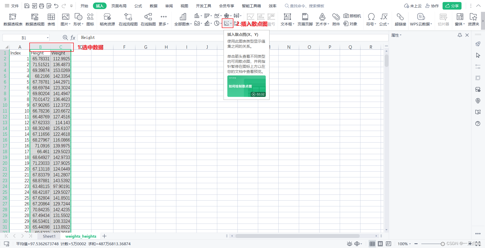
一、利用WPS进行线性回归分析

1、20组数据

选中两组数据，插入散点图

更改数据为前20组

 进行线性回归分析

选中散点图，点击图表元素，选中趋势线

 显示回归方程和R平方值

选中回归线，点击趋势线，选中显示公式和R平方值

获得数据

2、200组数据

将数据更改为使用前200组

 

获得数据

3、2000组数据

将数据更改为前2000组

获得数据

二、利用jupyter编程（不借助第三方库） 对数据进行线性回归分析

1、将数据文件上传（方便后续打开数据文件）

 2、添加代码

import pandas as pd
import numpy as np
import math
import matplotlib.pyplot as plt
#准备数据
p=pd.read_excel('weights_heights(身高-体重数据集).xls','weights_heights')
#读取20行数据
p1=p.head(20)
x=p1["Height"]
y=p1["Weight"]
# 平均值
x_mean = np.mean(x)
y_mean = np.mean(y)
#x（或y）列的总数（即n）
xsize = x.size
zi=((x-x_mean)*(y-y_mean)).sum()
mu=((x-x_mean)*(x-x_mean)).sum()
n=((y-y_mean)*(y-y_mean)).sum()
# 参数a b
a = zi / mu
b = y_mean - a * x_mean
#相关系数R的平方
m=((zi/math.sqrt(mu*n))**2)
# 这里对参数保留4位有效数字
a = np.around(a,decimals=4)
b = np.around(b,decimals=4)
m = np.around(m,decimals=4)
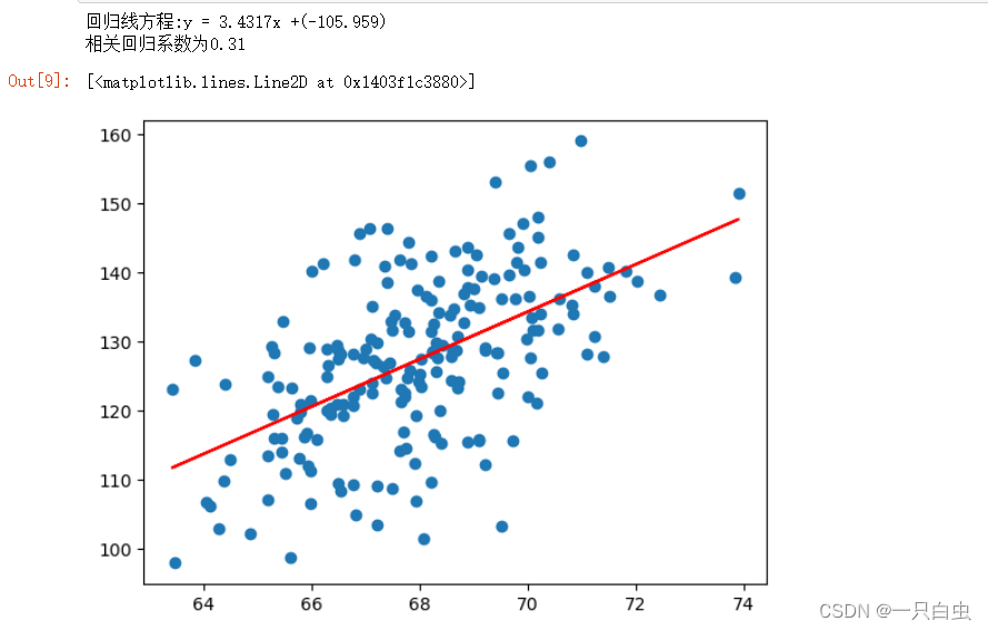
print(f'回归线方程:y = {a}x +({b})') 
print(f'相关回归系数为{m}')
#借助第三方库skleran画出拟合曲线
y1 = a*x + b
plt.scatter(x,y)
plt.plot(x,y1,c='r')

输出20组数据

3 、输出200组数据

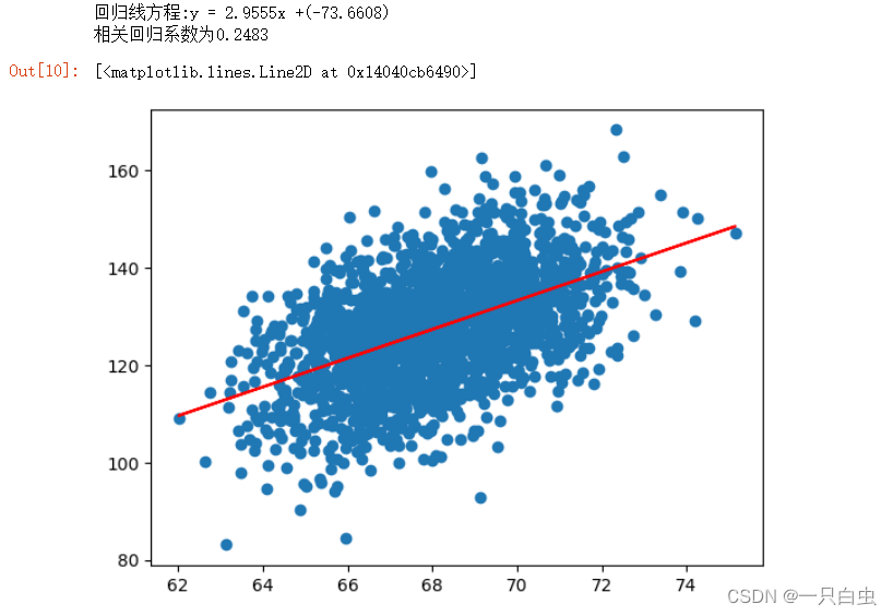
4、输出2000组数据

 5、利用pandas打开excel文件出现ImportError解决方法

错误原因：没有安装xlrd模块

解决方法：在Anaconda安装xlrd模块

激活虚拟环境

 安装xlrd模块

conda install -c anaconda xlrd

 三、借助skleran对数据进行线性回归分析

添加代码

# 导入所需的模块
import numpy as np
import pandas as pd
import matplotlib.pyplot as plt
from sklearn.linear_model import LinearRegression

p=pd.read_excel('weights_heights(身高-体重数据集).xls','weights_heights')
#读取数据行数
p1=p.head(20)
x=p1["Height"]
y=p1["Weight"]
# 数据处理
# sklearn 拟合输入输出一般都是二维数组，这里将一维转换为二维。
y = np.array(y).reshape(-1, 1)
x = np.array(x).reshape(-1, 1)
# 拟合
reg = LinearRegression()
reg.fit(x,y)
a = reg.coef_[0][0]     # 系数
b = reg.intercept_[0]   # 截距
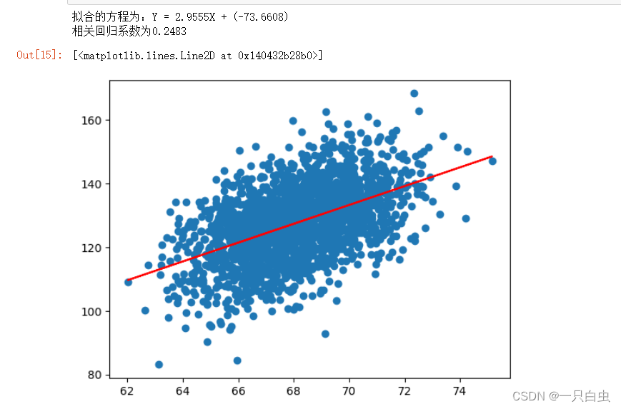
print('拟合的方程为：Y = %.4fX + (%.4f)' % (a, b))
c=reg.score(x,y)    # 相关系数
print(f'相关回归系数为%.4f'%c)

# 可视化
prediction = reg.predict(y)                # 根据高度，按照拟合的曲线预测温度值
plt.scatter(x,y)
y1 = a*x + b
plt.plot(x,y1,c='r')

20组数据

 200组数据

2000组数据

 总结

利用wps和jupyter解决线性回归问题得出的结果大致相同。在利用jupyter解决线性回归问题时，出现无法打开目标文件读取数据，利用网络查询最终解决问题。

参考资料

Python错误集锦：pandas读取excel提示ImportError

Excel和jupyter实现数据的线性回归