Matplotlib实用绘图技巧总结
在日常的业务数据分析 ,可视化是非常重要的步骤。这里总结了matplotlib常用绘图技巧,希望可以帮助大家更加更加高效的、美观的显示图表。作者:北山啦
Matplotlib 是 Python 的绘图库。 它可与 NumPy 一起使用,提供了一种有效的 MatLab 开源替代方案。 它也可以和图形工具包一起使用,如 PyQt 和wxPython。
推荐阅读:
matplotlib实用绘图技巧总结
Python 数据可视化–Seaborn绘图总结1
Python数据可视化–Seaborn绘图总结2
Tableau数据分析-Chapter01条形图、堆积图、直方图
Tableau数据分析-Chapter02数据预处理、折线图、饼图
Tableau数据分析-Chapter03基本表、树状图、气泡图、词云
Tableau数据分析-Chapter04标靶图、甘特图、瀑布图
Tableau数据分析-Chapter05数据集合并、符号地图
Tableau数据分析-Chapter06填充地图、多维地图、混合地图
Tableau数据分析-Chapter07多边形地图和背景地图
Tableau数据分析-Chapter08数据分层、数据分组、数据集
Tableau数据分析-Chapter09粒度、聚合与比率
Tableau数据分析-Chapter10 人口金字塔、漏斗图、箱线图
Tableau中国五城市六年PM2.5数据挖掘
文章目录
pip3 install matplotlib -i https://pypi.tuna.tsinghua.edu.cn/simple
import matplotlib.pyplot as plt
显示中文
借助全局参数配置字典rcParams,只需要在代码开头,添加如下两行代码即可
plt.rcParams['font.sans-serif'] = ['SimHei']
plt.rcParams['axes.unicode_minus'] = False
同时还可以设置字体,常见字体:
font.family  字体的名称
sans-serif   西文字体(默认)
SimHei       中文黑体
FangSong     中文仿宋`在这里插入代码片`
YouYuan      中文幼圆
STSong       华文宋体
Kaiti        中文楷体
LiSu         中文隶书
字体风格
plt.rcParams["font.style"] = "italic"
矢量图设置
在默认设置的matplotlib中图片分辨率不是很高,可以通过设置矢量图的方式来提高图片显示质量
%matplotlib inline
%config InlineBackend.figure_format = 'svg'
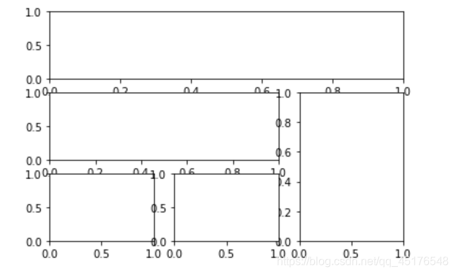
绘制子图
画图时,show()是个阻塞函数总是要放在最后,它阻止命令继续往下运行
- plt.subplot2grid()
plt.subplot2grid((3,3),(0,0),colspan=3)
plt.subplot2grid((3,3),(1,0),colspan=2)
plt.subplot2grid((3,3),(1,2),rowspan=2)
plt.subplot2grid((3,3),(2,0))
plt.subplot2grid((3,3),(2,1))
plt.show()
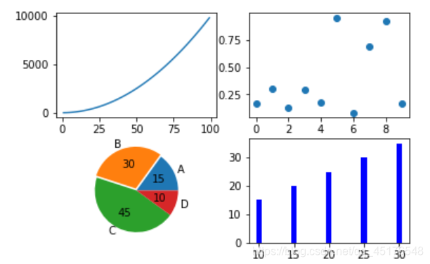
2. plt.subplot()
import numpy as np
import pandas as pd
import matplotlib.pyplot as plt
# 画第1个图:折线图
x=np.arange(1,100)
plt.subplot(221)
plt.plot(x,x*x)
# 画第2个图:散点图
plt.subplot(222)
plt.scatter(np.arange(0,10), np.random.rand(10))
# 画第3个图:饼图
plt.subplot(223)
plt.pie(x=[15,30,45,10],labels=list('ABCD'),autopct='%.0f',explode=[0,0.05,0,0])

# 画第4个图:条形图
plt.subplot(224)
plt.bar([20,10,30,25,15],[25,15,35,30,20],color='b')
plt.show()
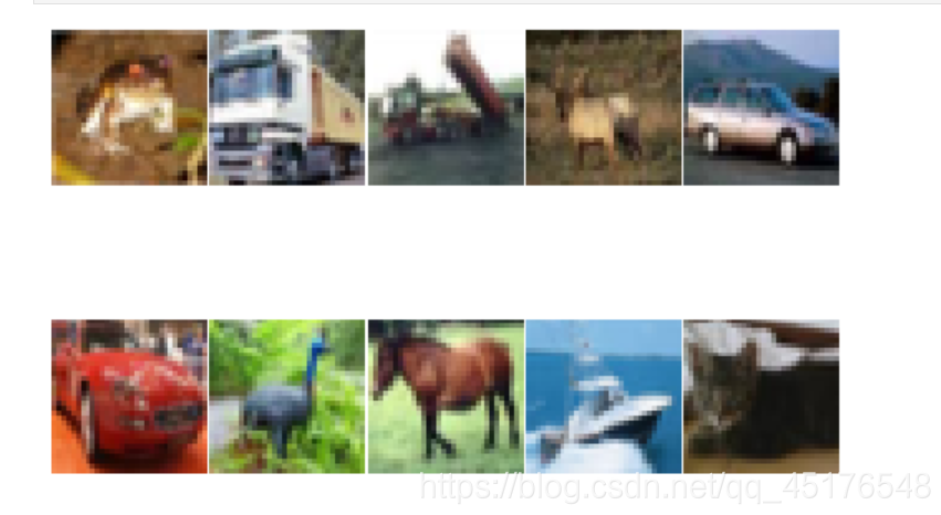
matplotlib绘图设置不显示边框、坐标轴
对于有些图形我们希望通过隐藏坐标轴来显得更加美观
plt.xticks([])
plt.yticks([])
ax = plt.subplot(2,5,1)
# 去除黑框
ax.spines['top'].set_visible(False)
ax.spines['right'].set_visible(False)
ax.spines['bottom'].set_visible(False)
ax.spines['left'].set_visible(False)
实例:
#author:https://beishan.blog.csdn.net/
import matplotlib.pyplot as plt
for i in range(0,10):
    fig = plt.gcf()
    fig.set_size_inches(12,6)
    ax = plt.subplot(2,5,i+1)
    # 去除坐标轴
    plt.xticks([])
    plt.yticks([])

    # 去除黑框
    ax.spines['top'].set_visible(False)
    ax.spines['right'].set_visible(False)
    ax.spines['bottom'].set_visible(False)
    ax.spines['left'].set_visible(False)
    # 设置各个子图间间距
    plt.subplots_adjust(left=0.10, top=0.88, right=0.65, bottom=0.08, wspace=0.02, hspace=0.02)
    ax.imshow(Xtrain[i],cmap="binary")
提高分辨率
如果感觉默认生成的图形分辨率不够高,可以尝试修改 dpi 来提高分辨率
plt.figure(figsize = (7,6),dpi =100)
设置绘图风格
有时我们会觉得matplotlib默认制作出来的图片太朴素了,不够高级,其实开发者也内置了几十种主题让我们自己选择,只要使用plt.style.use(‘主题名’)指定主题即可
plt.style.use('ggplot')
常用的样式有
Solarize_Light2
_classic_test_patch
bmh
classic
dark_background
fast
fivethirtyeight
ggplot
grayscale
seaborn
seaborn-bright
seaborn-colorblind
seaborn-dark
seaborn-dark-palette
seaborn-darkgrid
seaborn-deep
seaborn-muted
seaborn-notebook
seaborn-paper
seaborn-pastel
seaborn-poster
seaborn-talk
seaborn-ticks
seaborn-white
seaborn-whitegrid
tableau-colorblind10
添加标题
plt.title("2020-2021北山啦粉丝数增长图")
显示网格
plt.grid()
plt.grid(color='g',linewidth='1',linestyle='-.')
图例设置
plt.legend(["2020","2021"],loc="best")
也可以给图例添加标题
plt.plot([1,3,5,7],[4,9,6,8],"ro--")
plt.plot([1,2,3,4], [2,4,6,8],"gs-.")
plt.legend(["2020","2021"],loc="best",title="标题")
plt.title("2020-2021北山啦粉丝数增长图")
添加公式
有时我们在绘图时需要添加带有数学符号、公式的文字,
plt.text(11000,0.45,r'拟合曲线为$f(x) = x^2-4x+0.5$')
图形交互设置
jupyter中的魔法方法
%matplotlib notebook 弹出可交互的matplotlib窗口
%matplotlib qt5 弹出matplotlib控制台
%matplotlib inline 直接嵌入图表,不需要使用plt.show()
保存图片
plt.savefig("pic.png",dpi=100,bbox_inches="tight")
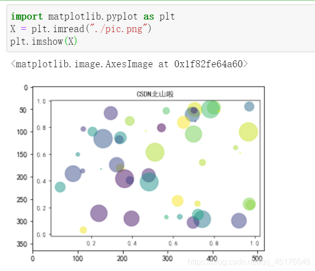
读取图片
- 方法一
from PIL import Image
image = Image.open("./pic.png")
image.show()
- 方法二
import matplotlib.pyplot as plt
X = plt.imread("./pic.png")
plt.imshow(X)
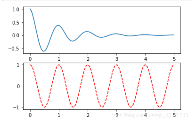
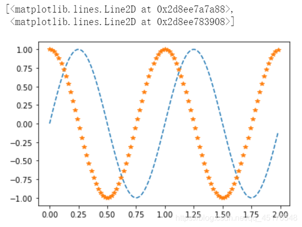
条形图
def f(t):
    return np.exp(-t) * np.cos(2*np.pi*t)
a = np.arange(0,5,0.02)

plt.subplot(211)
plt.plot(a,f(a))

plt.subplot(212)
plt.plot(a,np.cos(2*np.pi*a),'r--')

plt.show()
b = np.arange(0,2,0.02)
plt.plot(b,np.sin(2*np.pi*b),'--',b,np.cos(2*np.pi*b),"*")
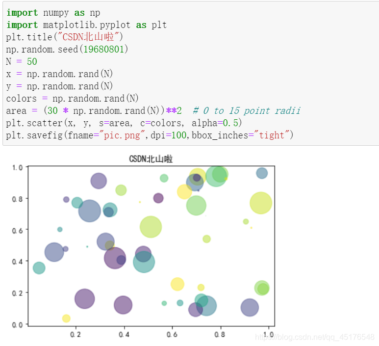
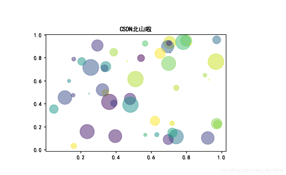
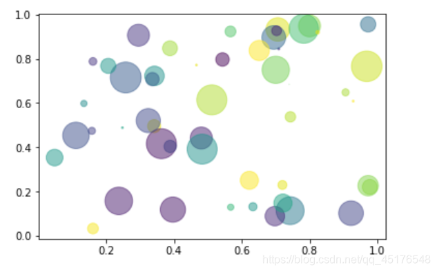
散点图
import numpy as np
import matplotlib.pyplot as plt

# Fixing random state for reproducibility
np.random.seed(19680801)


N = 50
x = np.random.rand(N)
y = np.random.rand(N)
colors = np.random.rand(N)
area = (30 * np.random.rand(N))**2  # 0 to 15 point radii

plt.scatter(x, y, s=area, c=colors, alpha=0.5)
plt.show()
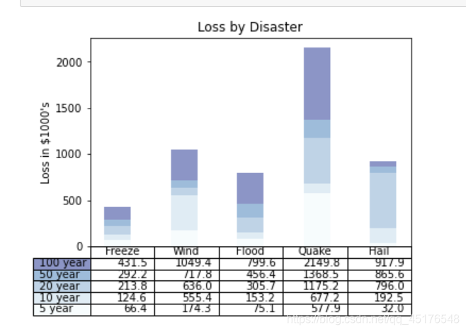
带表格的图形
import numpy as np
import matplotlib.pyplot as plt


data = [[ 66386, 174296,  75131, 577908,  32015],
        [ 58230, 381139,  78045,  99308, 160454],
        [ 89135,  80552, 152558, 497981, 603535],
        [ 78415,  81858, 150656, 193263,  69638],
        [139361, 331509, 343164, 781380,  52269]]

columns = ('Freeze', 'Wind', 'Flood', 'Quake', 'Hail')
rows = ['%d year' % x for x in (100, 50, 20, 10, 5)]

values = np.arange(0, 2500, 500)
value_increment = 1000

# Get some pastel shades for the colors
colors = plt.cm.BuPu(np.linspace(0, 0.5, len(rows)))
n_rows = len(data)

index = np.arange(len(columns)) + 0.3
bar_width = 0.4

# Initialize the vertical-offset for the stacked bar chart.
y_offset = np.zeros(len(columns))

# Plot bars and create text labels for the table
cell_text = []
for row in range(n_rows):
    plt.bar(index, data[row], bar_width, bottom=y_offset, color=colors[row])
    y_offset = y_offset + data[row]
    cell_text.append(['%1.1f' % (x / 1000.0) for x in y_offset])
# Reverse colors and text labels to display the last value at the top.
colors = colors[::-1]
cell_text.reverse()

# Add a table at the bottom of the axes
the_table = plt.table(cellText=cell_text,
                      rowLabels=rows,
                      rowColours=colors,
                      colLabels=columns,
                      loc='bottom')

# Adjust layout to make room for the table:
plt.subplots_adjust(left=0.2, bottom=0.2)

plt.ylabel("Loss in ${0}'s".format(value_increment))
plt.yticks(values * value_increment, ['%d' % val for val in values])
plt.xticks([])
plt.title('Loss by Disaster')

plt.show()
模板
from matplotlib import pyplot as plt
import random
from pylab import mpl

# 设置中文显示
mpl.rcParams["font.sans-serif"] = ["SimHei"]
mpl.rcParams["axes.unicode_minus"] = False

x = range(60)
y_shanghai = [random.uniform(15, 18) for i in x]
y_beijing = [random.uniform(1, 3) for i in x]

# 设置图像大小及清晰度
plt.figure(figsize=(20, 8), dpi=80)

# 绘制图像
plt.plot(x, y_shanghai, label="上海")
plt.plot(x, y_beijing, color="r", linestyle="--", label="北京")

x_ticks_label = ["11点{}分".format(i) for i in x]
y_ticks = range(40)
x_ticks = x[::5]

# 设置坐标轴刻度
plt.xticks(x_ticks, x_ticks_label[::5])
plt.yticks(y_ticks[::5])

# 设置网格
plt.grid(True, linestyle="--", alpha=1)

# 设置坐标轴含义
plt.xlabel("时间")
plt.ylabel("温度")
plt.title("中午11点到12点某城市的温度变化图", fontsize=20)

# 添加图例
plt.legend(loc="best")

# 图像保存
plt.savefig("./test.png")

# 展示图像
plt.show()
推荐阅读:
Tableau数据分析-Chapter01条形图、堆积图、直方图
Tableau数据分析-Chapter02数据预处理、折线图、饼图
Tableau数据分析-Chapter03基本表、树状图、气泡图、词云
Tableau数据分析-Chapter04标靶图、甘特图、瀑布图
Tableau数据分析-Chapter05数据集合并、符号地图
Tableau数据分析-Chapter06填充地图、多维地图、混合地图
Tableau数据分析-Chapter07多边形地图和背景地图
Tableau数据分析-Chapter08数据分层、数据分组、数据集
Tableau数据分析-Chapter09粒度、聚合与比率
Tableau数据分析-Chapter10 人口金字塔、漏斗图、箱线图
Tableau中国五城市六年PM2.5数据挖掘

到这里就结束了,如果对你有帮助,欢迎点赞关注,你的点赞对我很重要。作者:北山啦

AtomGit 是由开放原子开源基金会联合 CSDN 等生态伙伴共同推出的新一代开源与人工智能协作平台。平台坚持“开放、中立、公益”的理念,把代码托管、模型共享、数据集托管、智能体开发体验和算力服务整合在一起,为开发者提供从开发、训练到部署的一站式体验。
更多推荐


 39
39 0
0- 0


 已为社区贡献8条内容

所有评论(0)